Assembly, and why the matrix is nearly empty

Lead figure

Each element touches few neighbours, so the global system is sparse — which is the only reason any of this is tractable.

What assembly actually does

Every element in a finite element mesh has its own small stiffness matrix, assembled from integrals over that element's geometry and material properties. For a quadrilateral with four nodes, that local matrix is 8 × 8 in two-dimensional elasticity; for a twenty-node hexahedron it is 60 × 60. The assembly step maps each of those local matrices into the correct rows and columns of the global system, governed by a connectivity table that records which global degrees of freedom belong to which element. Where two elements share a node, their contributions to the rows and columns associated with that node are summed. Nothing more exotic than that: scatter, and accumulate.

The result is a global stiffness matrix K of dimension N × N, where N is the total number of degrees of freedom — easily in the millions for an industrial mesh. If every node interacted with every other, K would be dense and the memory cost alone would make the method unusable at any practical scale. It is not dense, because physics is local.

Why almost every entry is zero

A node in a finite element mesh only communicates directly with the nodes it shares an element with. In a three-dimensional mesh of tetrahedra, a typical interior node touches perhaps a dozen or so neighbours, regardless of how large N grows. The ratio of non-zero entries to the total N² entries therefore shrinks as N grows: a matrix with one million degrees of freedom might have fewer than fifty non-zeros per row, giving a fill fraction below 0.005 per cent. This is what practitioners mean by sparse matrix — not merely thin, but structurally sparse in a way that reflects the neighbourhood structure of the mesh.

The sparsity pattern is fixed before any numbers are computed. Software typically performs a symbolic assembly pass — traversing the connectivity table to identify which entries will be non-zero — and allocates only those positions. The numerical values are filled in afterward. Storing K in compressed sparse row or compressed sparse column format then costs memory proportional to the number of non-zeros, not to N², and matrix–vector products cost similarly. Direct and iterative solvers alike exploit this: a sparse Cholesky or LDLT factorisation, for instance, fills in additional non-zeros during factorisation, but the fill remains manageable when the matrix is first reordered by algorithms such as nested dissection or Cuthill–McKee.

What the pattern costs

The nonzero pattern is fixed by the mesh connectivity, and the ordering of the nodes decides how much fill-in a direct factorisation will generate.

The practical consequence is stark. Without sparsity, a structural analysis with 10⁶ degrees of freedom would require storing 8 terabytes in double precision for a dense matrix. With sparsity and roughly 40 non-zeros per row, the same system fits in a few hundred megabytes — the difference between impossible and routine.

For a quadrilateral with four nodes, that local matrix is 8 × 8 in two-dimensional elasticity;

What can go wrong

Assembly errors are among the most common implementation mistakes in finite element codes. An incorrect connectivity table maps local degrees of freedom to the wrong global positions, producing a matrix that is assembled without error but is quietly wrong. The symptoms are indistinguishable from a material or boundary-condition error: solutions that are continuous but incorrect, or convergence to the wrong answer. The standard check is to verify against a problem with a known analytical solution and inspect whether the error converges at the expected rate with mesh refinement — a flat or erratic convergence curve almost always points upstream, toward assembly or shape-function implementation, before anything else.

A subtler failure occurs when two element types with incompatible degree-of-freedom numbering are joined — a quadratic triangle meeting a linear quadrilateral, for instance — and the connectivity table silently drops the midside nodes. The assembled matrix is legal and sparse, but the interface is a displacement discontinuity. Element shape and formulation must be compatible, or assembly propagates the mismatch throughout the solve invisibly.

The sparsity of the global matrix is not a convenience; it is the load-bearing fact on which the tractability of large-scale computation rests.

Sparsity at scale

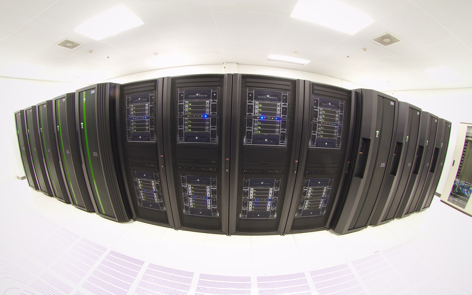
A million-equation system is routine only because each row holds a handful of entries; the same structure is what lets the problem be split across processes.

Photo: Dutch national supercomputer "Huygens" - 8183833489 · Wikimedia Commons