Cut it into pieces
A continuous body has infinitely many answers
Discretise the continuum, sum the local physics, solve once: the move that launched a half-century of computational mechanics.
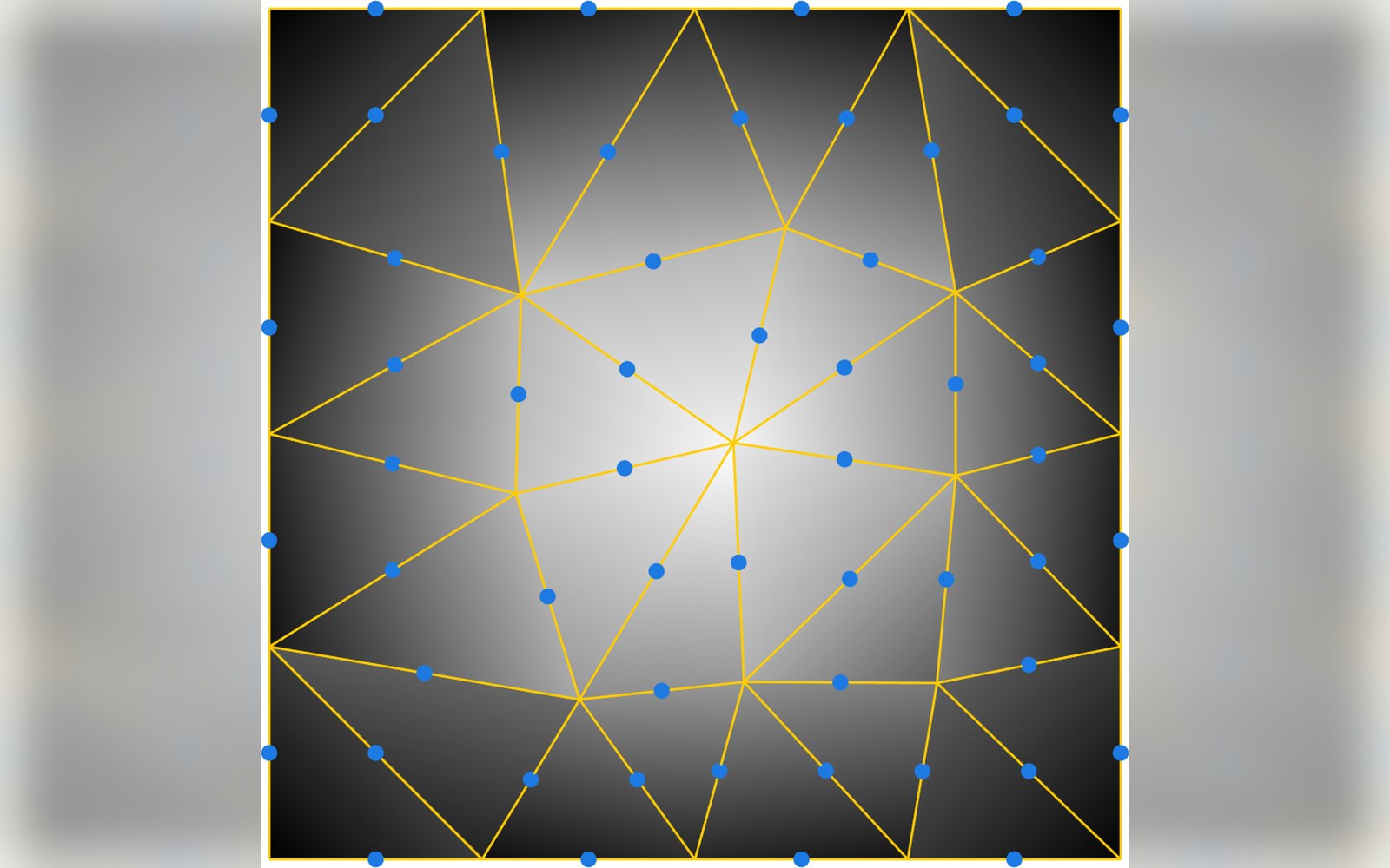
The finite element method came out of aircraft structures in the 1950s and its central move — elements, local physics, one assembled sparse system — has not changed.
Photo: Triangulation with edge midpoints · Wikimedia CommonsThe problem that forces the method
A continuous elastic solid has infinitely many degrees of freedom. Stress and displacement vary from point to point across a domain whose shape is usually irregular, whose loads are unevenly distributed, and whose boundary conditions mix prescribed displacements against prescribed tractions in ways that resist any closed-form treatment. Classical theory can hand you exact solutions for a handful of idealised geometries — a sphere under uniform pressure, a half-space with a point load — but the moment the geometry departs from those ideals, the continuum wins. You cannot write down the answer.
The finite element method's central manoeuvre is to stop trying. Replace the infinite-dimensional problem with a finite one by dividing the domain into small subregions — the elements — and approximating the unknown field inside each one using a small set of basis functions anchored to the element's nodes. The unknown is no longer a function over a continuous domain; it is a finite vector of nodal values, and everything else — strains, stresses, reactions — follows from those values through the approximation. What was intractable becomes a linear algebra problem, and linear algebra has solvers.
This is not a new idea in the history of approximation, but its systematic application to structural mechanics crystallised in the 1950s. The 1956 paper by Turner, Clough, Martin and Topp, working at Boeing and Berkeley, derived stiffness matrices for triangular and rectangular plane-stress elements from direct physical reasoning, and demonstrated convergence on aircraft panel problems. Ray W. Clough coined the phrase "finite element method" in 1960, and John Argyris, working in parallel in Stuttgart, developed a similarly general framework using energy principles. Olgierd Zienkiewicz later at Swansea turned the method into a systematic discipline through his textbook, whose first edition appeared in 1967 and whose successive editions tracked three decades of theoretical development.

Each element contributes a small dense matrix into the rows and columns its own nodes own. Nothing else in the global system is touched, which is where the sparsity comes from.
Elements, assembly, and why the matrix stays sparse
Pick up a single element. Its geometry is defined by a small number of nodes — three for a linear triangle, eight for a trilinear hexahedron — and the displacement field inside is written as a combination of shape functions, one per node, each equal to unity at its own node and zero at all others. Integrate the strain energy over the element, minimise with respect to nodal displacements, and you recover the element stiffness matrix: a small, dense matrix relating forces at that element's nodes to displacements at those same nodes. The local physics is contained entirely in that matrix.
Assembly is the step that turns a collection of local matrices into a global system. Each node belongs to several elements; the global stiffness matrix is accumulated by adding each element's contribution into the rows and columns corresponding to its nodes. The result is a matrix whose size equals the total number of degrees of freedom — potentially millions in an industrial mesh — but which is almost entirely empty. Each equation couples a node only to its immediate neighbours, so the global stiffness matrix is sparse, with nonzero entries confined to a narrow band or a structured pattern that direct solvers can exploit through sparse factorisation, or that iterative solvers can multiply through cheaply.
What was intractable becomes a linear algebra problem, and linear algebra has solvers.
This sparsity is not incidental. It is the structural consequence of local support — the fact that each shape function is nonzero over only the elements that share its node — and it is what makes the finite element method computationally viable at scale. A dense global matrix for a million-degree-of-freedom problem would be unreachable; the sparse equivalent is solved routinely.
From structures to fluids, and the things that did not change
The method spread from structural mechanics into heat conduction, electromagnetics, and eventually fluid dynamics, carried by the recognition that the same weighted-residual framework — the Galerkin method — applies to any partial differential equation that can be cast in weak form. For fluids the governing equations are the Navier–Stokes equations rather than the equations of linear elasticity, the unknowns are velocity and pressure rather than displacement, and the nonlinearity introduced by the convective term demands iterative linearisation strategies that structural mechanics rarely requires. Turbulence modelling adds further closure equations whose accuracy is the subject of ongoing research rather than settled theory.
Yet the architecture did not change. There are still elements, still local integrals over those elements evaluated by Gaussian quadrature ↗, still an assembled sparse system solved at each iteration, still node-based unknowns whose meaning follows from the choice of shape function. The finite volume method, dominant in many CFD codes, is a different discretisation philosophy, but its practical implementation shares most of the same infrastructure — mesh, connectivity, sparse linear system, iterative solver — and the concerns that govern accuracy are recognisably parallel: mesh quality, solution-adaptive refinement, verification of convergence rates.
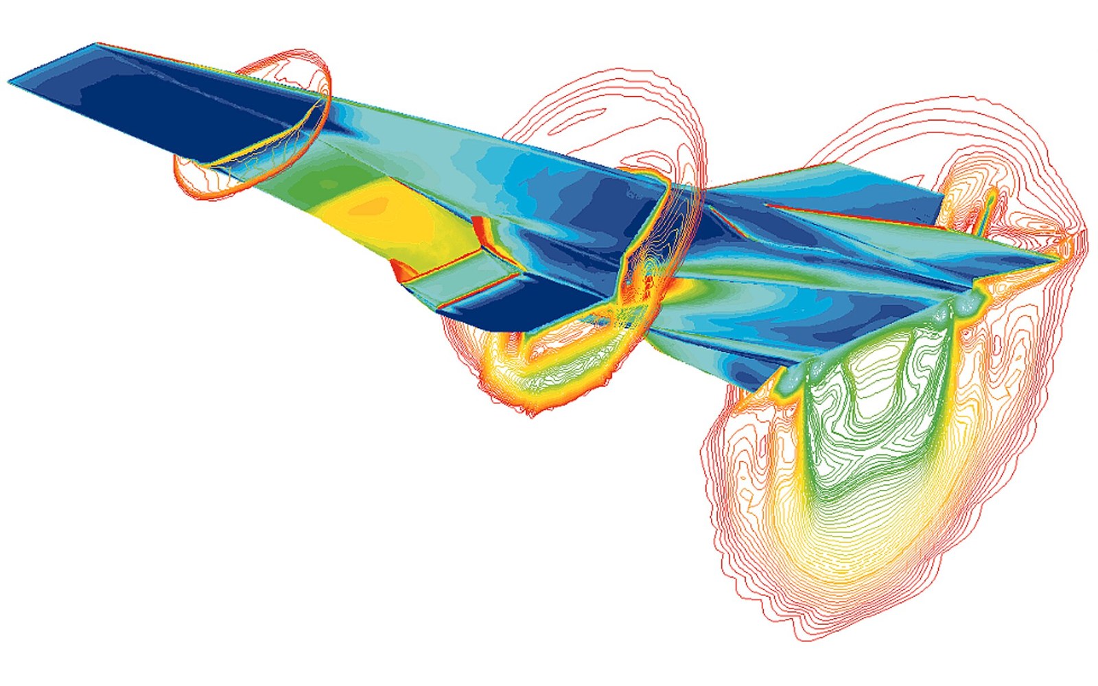
The same weighted-residual framework transferred to the Navier–Stokes equations, with velocity and pressure replacing displacement and a convective term that has to be linearised at every iteration.
Photo: X-43A (Hyper - X) Mach 7 computational fluid dynamic (CFD) · Wikimedia CommonsOn the verification side, the method of manufactured solutions — prescribing an exact solution, deriving the body force it implies, running the code, checking whether the error falls at the expected algebraic rate as the mesh is refined — became the standard self-consistency test precisely because the theoretical error bounds from finite element analysis give a quantitative prediction to check against. Convergence at the wrong rate signals either a coding error or a failure of the mesh to satisfy the smoothness assumptions the error estimate requires. Neither outcome is acceptable, and neither is revealed by running a single mesh.
What the founding generation established in the 1950s, and what Zienkiewicz's textbook disseminated internationally, was not merely a useful approximation scheme but a coherent theory: existence and uniqueness of the discrete solution inherited from the continuous problem under appropriate conditions, error bounds in energy norms tied to element size and polynomial degree, and systematic strategies for improving accuracy through refinement or through raising the polynomial order. The mathematical foundations ↗ — variously attributed to work by Strang and Fix, among others — arrived in published form by the early 1970s and transformed the method from an engineering heuristic into a branch of numerical analysis with provable guarantees. Those guarantees come with conditions, and knowing which conditions fail in a given problem is most of what applied finite element analysis actually demands.