Direct against iterative
RANS, LES and DNS — three bargains
Turbulence is unsolved physics. Every simulation approach is a deal: compute less, model more — or pay the full price and still get only one realisation.
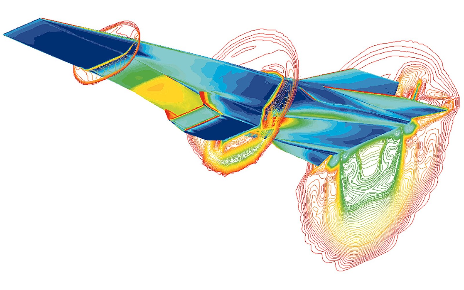
Turbulence is the open problem, and each approach trades cost against how much of it is modelled rather than resolved.
Photo: X-43A (Hyper - X) Mach 7 computational fluid dynamic (CFD) · Wikimedia CommonsThe thing you are actually trading
Turbulent flow contains eddies at every scale from the geometry-spanning large structures down to the Kolmogorov microscale, where kinetic energy finally dissipates as heat. The ratio of the largest to the smallest scale goes as Re³/⁴, where Re is the Reynolds number. A pipe flow at Re = 10⁶ has roughly four to five orders of magnitude separating the two ends of that spectrum. Resolving every eddy everywhere — Direct Numerical Simulation — means a computational mesh that scales as Re⁹/⁴ in three dimensions, and a time-step that scales similarly. That is not a warning; it is the cost estimate implied by the Navier–Stokes equations themselves, and it is why DNS of even modest Reynolds numbers remains a research instrument rather than an engineering tool.
Every other approach avoids that cost by deciding that some portion of the turbulent motion will be modelled rather than computed. The three canonical bargains are DNS, Large Eddy Simulation and Reynolds-Averaged Navier–Stokes, listed in descending order of what they actually resolve and ascending order of what they require you to believe.
DNS — the full price
DNS resolves every turbulent scale directly on the mesh. There is no turbulence model; the only modelling is in the discretisation scheme and time integrator themselves, which introduces truncation error rather than physical closure assumptions. The requirement is that the mesh spacing everywhere satisfies Δx ≲ η, where η is the Kolmogorov length scale. At channel flow conditions explored in benchmark computations — canonical cases at Reτ of a few thousand — this demands meshes running to tens of billions of cells and wall-clock times that fill supercomputer allocations.
What DNS delivers in return is unique: it provides the full velocity and pressure fields at every point in space and time with no modelled physics in the turbulence. That makes it the reference against which closure models are tested, and its outputs have been used to derive improved model coefficients since the 1980s. The first DNS of turbulent channel flow by Kim, Moin and Moser in 1987 is the canonical example. The raw data from that class of calculation — mean profiles, Reynolds stress budgets, spectra — are the empirical constants that populate every RANS model in industrial codes today.
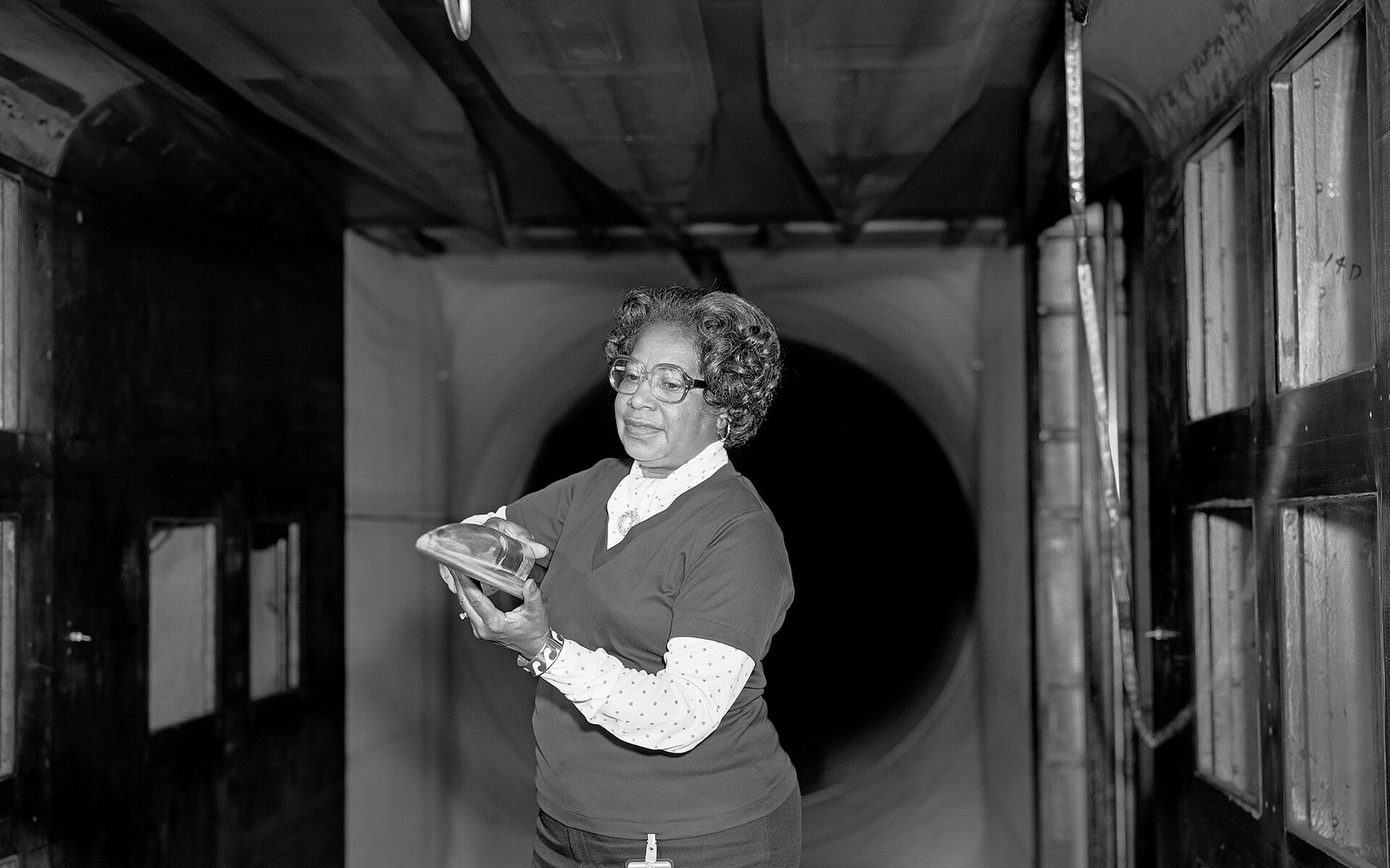
Wind tunnel data is what a turbulence model is calibrated and judged against; the model is not an independent source of truth.
Photo: Mary Jackson in a wind tunnel with a model at NASA Langley · Wikimedia CommonsThe honest limitation is scope. DNS is not, and in most interpretations cannot become, an engineering method for high-Reynolds-number external aerodynamics or industrial pipe networks. It is a precision instrument for controlled canonical geometries.
A pipe flow at Re = 10⁶ has roughly four to five orders of magnitude separating the two ends of that spectrum.
LES — the intermediate bargain
Large Eddy Simulation resolves the large, energy-carrying eddies directly and models only the sub-grid scales — the motions smaller than the local filter width, which is typically the mesh spacing. The argument for doing this is that large eddies are geometry-dependent and anisotropic, so they should be computed; small eddies are more nearly isotropic and universal, so a generic model for them is more defensible than a model for everything.
The sub-grid scale model — the most widely used being Smagorinsky's algebraic eddy-viscosity formulation from 1963 — adds a dissipation that mimics the energy cascade to scales below the filter. Dynamic versions, developed by Germano and colleagues in 1991, compute the model coefficient locally from the resolved field, removing the need to set it by hand. These are real improvements, but the sub-grid model is still a model: it is wrong in regions of strong anisotropy such as the near-wall layer, and it cannot recover information lost below the filter.
The practical consequence is that LES is expensive in the near-wall region at high Reynolds numbers. The required resolution there scales roughly as Re², which drives cost toward DNS territory for external aerodynamics at flight conditions. Wall-modelled LES replaces the near-wall resolution requirement with a separate model — often a RANS treatment near the wall — trading accuracy for affordability. This hybrid idea is also the basis of Detached Eddy Simulation ↗ and its variants, which use RANS in the attached boundary layer and switch to LES in separated regions where it matters most. The switch criterion is itself an approximation, and the interface between the two treatments is an active research concern.
LES is the method of choice for problems where unsteady large-scale structures genuinely control the physics — combustors, bluff-body wakes, acoustic sources — and where RANS has historically failed. Its cost is prohibitive for parametric sweeps across many operating conditions, which is exactly where industry needs answers.
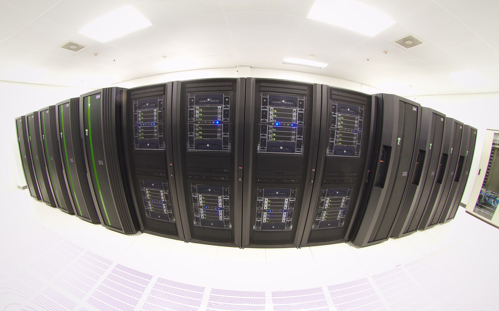
Resolving every scale means a grid count that rises steeply with Reynolds number, which is why the choice is made on budget.
Photo: Dutch national supercomputer "Huygens" - 8183833489 · Wikimedia CommonsRANS — the affordable fiction
Reynolds-Averaged Navier–Stokes averages the flow equations in time (or in an ensemble sense), producing equations for the mean velocity and pressure. The averaging introduces the Reynolds stress tensor — six unknowns — for which there is no closed equation. Everything that follows is a closure model, and there are many: the k-ε family, k-ω and its SST variant due to Menter, the Spalart–Allmaras one-equation model, full second-moment closures. None of them can be derived rigorously from the Navier–Stokes equations; they are calibrated against experimental data and DNS results for canonical flows.
RANS is fast. A steady RANS calculation of an aircraft configuration or a turbomachinery stage is entirely tractable on contemporary hardware. That is why it dominates industrial practice. It is also wrong in a predictable set of circumstances: strongly separated flows, flows with significant streamline curvature, reattachment after a step, impinging jets. The eddy-viscosity assumption — that the Reynolds stresses are proportional to the mean strain rate — is not a physical law. It is a conjecture that works when the turbulence structure is locally in equilibrium with production and dissipation, and fails when it is not.
RANS validation is extensive and the failure modes are documented. The NASA Langley turbulence modelling resource, which collects comparison data for standard test cases, is the community's shared ledger for where each model succeeds and where it does not. Knowing that ledger is as important as knowing how to run the code.
Choosing a bargain
No single approach is universally correct. DNS is a research instrument. LES is appropriate when unsteady separated physics must be captured and budget permits. RANS is the workhorse — appropriately, because it is computationally tractable — and its failure modes must be part of the engineer's working knowledge rather than a footnote.
The meaningful question is not which method is best, but which bargain a given problem can afford, and whether the terms of that bargain are compatible with the accuracy the decision actually requires.