Nobody's Favourite Job, and Where the Answer Is Won

Lead figure

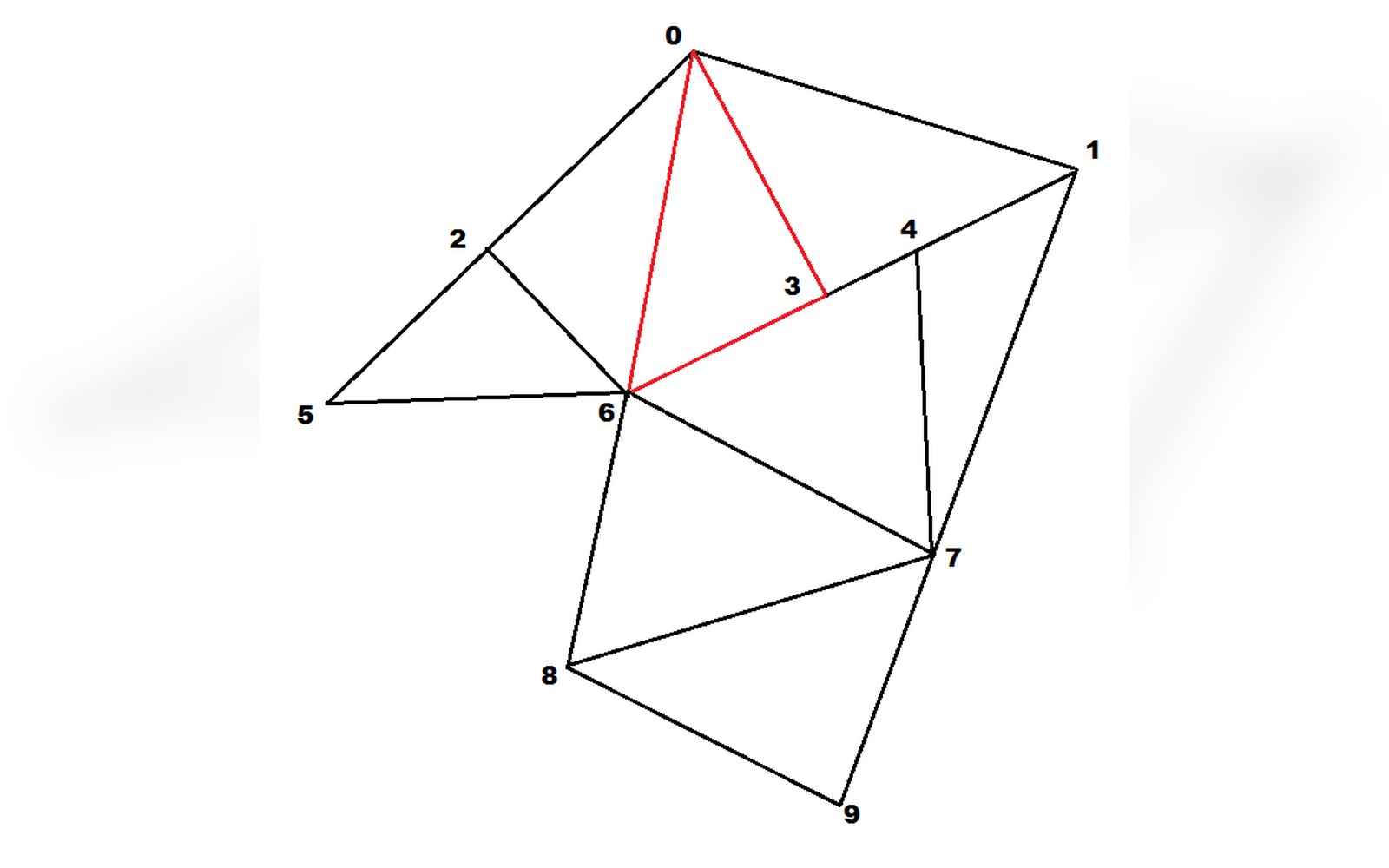
Meshing is where practitioners actually spend their time, and a badly shaped element poisons the solution around it.

Photo: Mesh FEM · Wikimedia Commons

The Hidden Cost of a Computation

Ask any practitioner how long a simulation takes, and you get two very different numbers: the wall-clock time the solver runs, and the human time spent before it starts. For most industrial problems, the second number is larger. A finite element computation on a gas-turbine casing or a ship hull does not fail because the conjugate-gradient iteration diverged or the turbulence model was mis-specified. It fails — or quietly produces a wrong answer — because someone extruded a boundary-layer mesh into a geometry that was never quite watertight, or because an automatic tetrahedral mesher placed slivers in the wake of a sharp trailing edge and nobody caught them before the run.

This is not a productivity complaint. It is a mathematical statement. The finite element method, as Ray W. Clough, John Argyris and Olgierd Zienkiewicz ↗ formalised it across the late 1950s and 1960s, is a machine for converting a continuous boundary-value problem into a finite system of equations. The quality of that conversion depends entirely on what the mesh looks like. The solver is solving the discretised system faithfully; if the discretised system is a poor approximation of the continuous one, faithfulness is not enough.

Why Badly Shaped Elements Poison the Solution

The mechanism is direct and quantifiable. Every element in an FEM mesh carries a map from the reference element — the canonical triangle or hexahedron on which the shape functions are defined — to its location in physical space. That map is governed by the Jacobian of the coordinate transformation. When an element is well-shaped, the Jacobian is well-conditioned and the map is nearly isometric. When an element is elongated, skewed, or — in the degenerate case — has a near-zero Jacobian anywhere in its interior, the map amplifies errors. Derivatives of the field variable are computed by inverting the Jacobian, so a Jacobian close to singular produces derivative errors that are locally enormous.

The error does not stay local. In an elliptic problem — Laplace, linear elasticity, Stokes flow — the solution at every point depends on every other point through the global stiffness matrix. A badly shaped element contaminates the entries it contributes to that matrix, and those entries couple to their neighbours. The condition number of the assembled system climbs. Iterative solvers stall or converge to the wrong answer; direct solvers give a result, but it may carry amplified floating-point error that the backward-error analysis of the factorisation does not warn you about.

Where the time goes

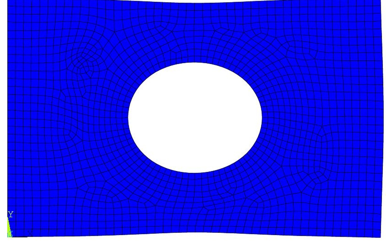
Geometry cleanup, feature suppression and local refinement are manual work, and they are what separates a mesh that converges from one that does not.

Photo: Meshing in Finite Element Analysis · Wikimedia Commons

The angular quality metrics — minimum interior angle, maximum interior angle, aspect ratio — are not aesthetic preferences. They enter the a priori error bounds for interpolation in $H^1$ directly, as Babuška and Aziz showed in their 1976 analysis of the finite element method: a maximum angle condition on triangulations is what is needed for optimal convergence. Let the minimum angle fall below roughly ten degrees in a two-dimensional triangulation and the interpolation error bound blows up, regardless of how fine the mesh is. Refinement cannot rescue a mesh that violates the angle condition uniformly, because the bound deteriorates faster than the element diameter shrinks.

if the discretised system is a poor approximation of the continuous one, faithfulness is not enough.

Where Practitioners Actually Spend Their Time

Geometry preparation is the first and usually the largest task. A CAD model assembled for manufacturing carries features — tiny fillets, slivers between nearly-coplanar faces, gaps at assembly interfaces — that are harmless for fabrication but catastrophic for a mesher. The mesher needs a watertight, consistently oriented surface; the CAD file rarely provides one without intervention. Defeaturing removes geometric detail whose length scale is far below the resolution the physics demands. A bolt-hole thread, for instance, matters nothing to a structural analysis seeking global deflection, but left in the model it forces the mesher to place elements with characteristic length of a fraction of a millimetre in a domain measured in metres, exploding the element count and wrecking aspect ratios in the surrounding region.

Once the geometry is clean, the choice between mesh topologies dominates the accuracy-versus-effort trade. Hexahedral elements, aligned with the flow or stress direction, are substantially more accurate per degree of freedom than unstructured tetrahedra — their tensor-product structure concentrates integration points efficiently, and their regular connectivity reduces condition number. But generating a high-quality all-hex mesh on an arbitrary geometry is genuinely hard: it reduces to a problem in global topology that no robust automatic algorithm has fully solved. Unstructured tet meshing is automatic and forgiving, fast on complex geometry, and the default choice in many industrial workflows, precisely because it trades some accuracy for a process that actually completes in a finite engineering lifetime.

The boundary layer deserves special attention in any viscous flow simulation. Near a wall, the velocity gradient is steep and the physics of turbulence — whether you are running RANS, LES or DNS — depends on resolving that gradient. Structured layers of highly anisotropic hexahedral or prismatic elements are extruded from the wall surface, with aspect ratios that may reach hundreds to one in the wall-normal direction. Inside each such element the Jacobian is large but the ratio between wall-normal and wall-tangential resolution is controlled by design, so the interpolation is accurate in the direction that matters. The pathology arises at corners and concave features, where prism layers collide and the mesher must insert a pyramid or a degenerate tet to close the gap — precisely the region where the flow is most complex and the element quality is worst.

Verification of a computation — the question of whether the mathematics was solved correctly — cannot be answered without a mesh convergence study. The standard practice is to run the same problem on a sequence of systematically refined meshes and check that the quantity of interest converges at the rate the element order predicts. The method of manufactured solutions sharpens this by providing an exact answer to compare against, so that convergence rate can be measured rather than inferred. A simulation that has not been checked this way has an unknown discretisation error, and an unknown discretisation error is an unknown total error.

Two families

Hexahedral meshes behave better under bending and plasticity; tetrahedral meshes can be generated automatically on almost any solid.

None of this is philosophically complicated. It is, however, stubbornly time-consuming, and the tools available — commercial preprocessors, open-source meshers such as Gmsh, Netgen, and OpenFOAM's snappyHexMesh — are powerful but still limited by the gap between what error estimates assume and what real geometry provides. The meshing problem will not be automated away by better algorithms alone, because the decisions that matter — what resolution the physics demands, where the geometry can be simplified, whether a feature needs resolution or removal — require physical judgment that the mesher does not possess. The solver gets the credit. The mesh is where the answer is actually built, or broken.