Where the theory stops and the mesher starts

Lead figure

Error estimates assume things about the mesh that real geometry rarely provides.

The gap nobody admits in the textbook

Finite element error theory is genuinely beautiful. For a second-order elliptic problem on a conforming mesh of degree-p elements, the energy norm error decreases like h^p, where h is the maximum element diameter — provided the solution is smooth enough and the elements are well-shaped enough to keep the Jacobian bounded. Zienkiewicz and Taylor's The Finite Element Method states this clearly, and the analysis behind it is rigorous. The problem is the word provided.

That bound requires that every element in the mesh satisfies an angle condition — no interior angles collapsing toward zero or stretching toward 180°. It also assumes that the mesh can be refined uniformly, that the domain boundary is approximated to the same order as the interior solution, and that no element is so distorted that its Jacobian changes sign. In academic test cases on square domains with manufactured solutions, all of these things are true by construction. On real geometry — a turbine blade trailing edge, a bolted joint fillet, a ship hull waterline — none of them is automatically satisfied, and no theorem guarantees they will be.

The meshing algorithm is where this burden lands. Automatic mesh generators, whether advancing-front or Delaunay-based, enforce angle bounds heuristically. They improve quality by local operations — edge swaps, node smoothing, topological reconnection — guided by quality metrics that correlate with the error bound but are not the error bound itself. When a surface has a sharp re-entrant corner, the local solution is singular: its derivatives blow up, the smoothness assumption fails, and the h^p convergence rate degrades regardless of what the mesher does. The analyst can know this and use local refinement or graded meshes to recover algebraic convergence, but only if they recognise that the estimate no longer applies globally.

Boundary layer meshes for viscous flow add another layer of mismatch. RANS and LES simulations require cells with aspect ratios that would fail every standard quality check — thin, flat hexahedra or prisms that satisfy the physics but violate the isotropy assumption baked into most error estimates. The theory for anisotropic elements exists, developed through the 1990s by researchers including Apel and Dobrowolski, but it is rarely what a mesh generator's quality report reflects.

The silent asterisk

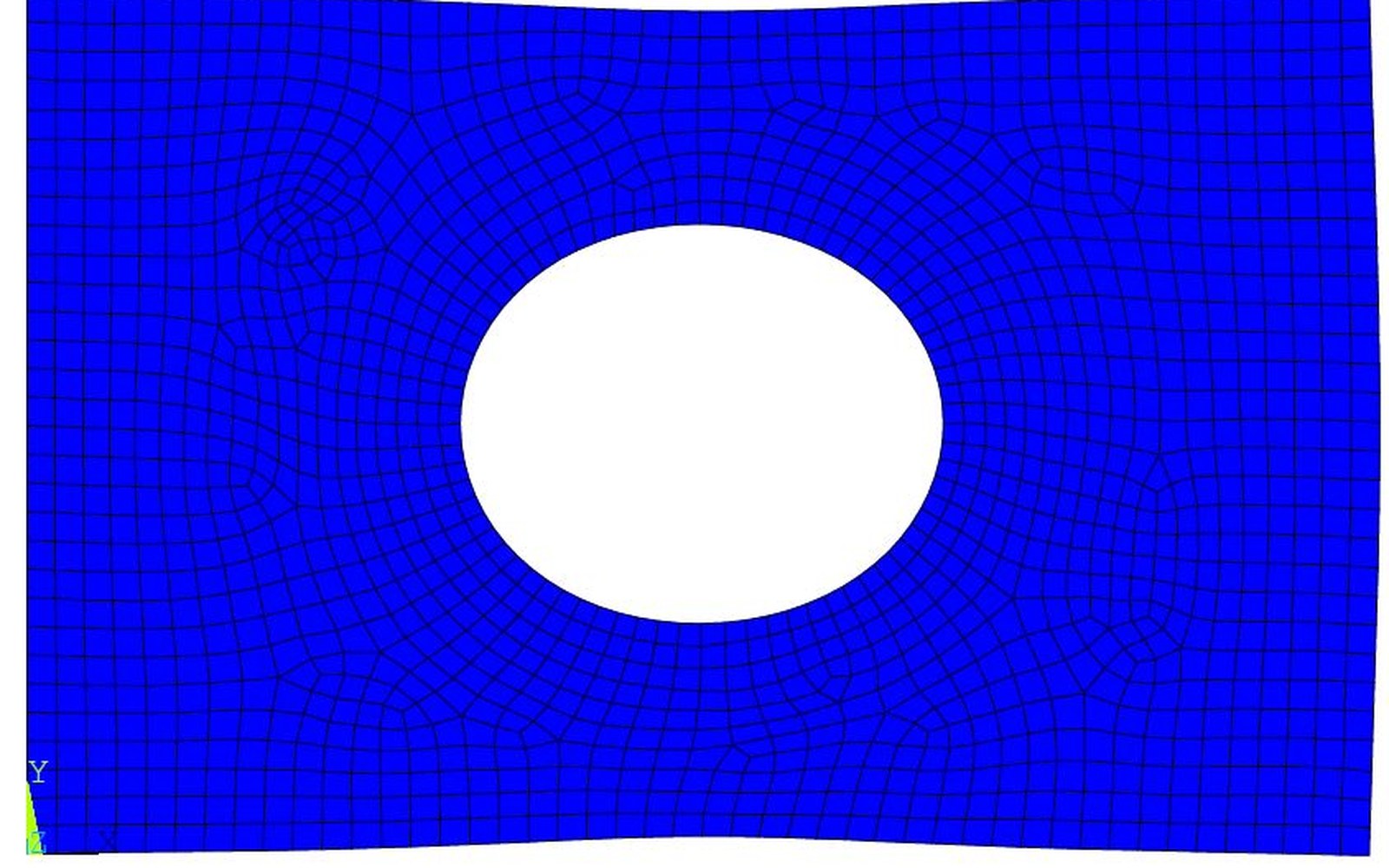
The bound assumes bounded angles, a smooth solution and uniform refinement. Real geometry supplies none of those by construction.

Photo: Meshing in Finite Element Analysis · Wikimedia Commons

The honest position is that error estimates from a 1972 paper describe a mathematical world the mesher approximates as faithfully as the geometry allows — which is sometimes well, and sometimes not at all. Knowing which situation you are in is the practitioner's job, and no convergence plot substitutes for understanding why the estimate was derived in the first place.

That bound requires that every element in the mesh satisfies an angle condition — no interior angles collapsing toward zero or stretching toward 180°.

Where it fails first

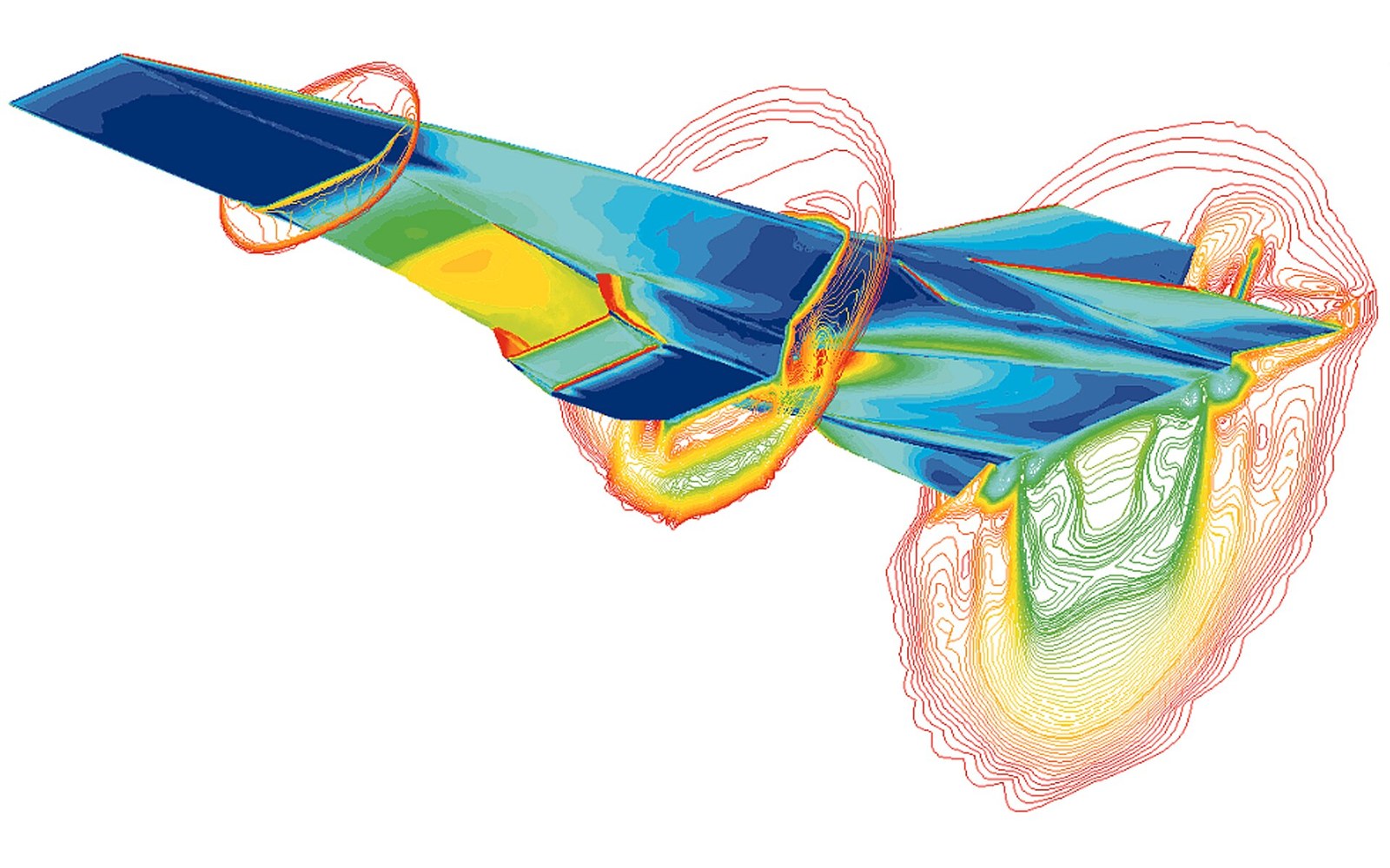
Near-wall meshes for viscous flow are anisotropic on purpose and fall outside the isotropy assumption most estimates carry.

Photo: X-43A (Hyper - X) Mach 7 computational fluid dynamic (CFD) · Wikimedia Commons