Nobody's favourite job
Why element shape governs accuracy
Aspect ratio, skew and Jacobian are not aesthetics: they enter the error bound directly.
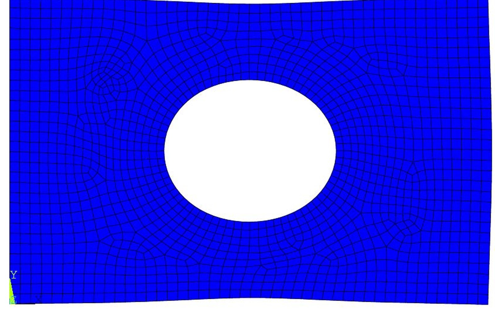
Aspect ratio, skew and Jacobian are not aesthetics: they enter the error bound directly.
Photo: Meshing in Finite Element Analysis · Wikimedia CommonsThe bound is not abstract
Error estimates in the finite element method are not reassuring platitudes about convergence in the limit. They are inequalities with explicit dependence on mesh geometry, and that dependence is multiplicative. The classical result, developed rigorously through the 1970s by Philippe Ciarlet and others building on work by Olgierd Zienkiewicz ↗, states roughly that the interpolation error is bounded by a product of two terms: a power of the element diameter h, and a constant that grows with the departure of the element from its ideal shape. Halving h buys nothing if the shape constant is climbing faster.
The precise form involves what Ciarlet called the "regularity" of a mesh family — a condition requiring that as h shrinks, the ratio of element diameter to the diameter of the largest inscribed sphere remains bounded. In plain terms: elements must not flatten or taper as they are refined. Ciarlet's 1978 monograph is the canonical reference for this derivation, and it makes clear that the shape condition is a hypothesis of the theorem, not a technicality to be waved away.
Three shape defects and what each one breaks
Aspect ratio is the ratio of the longest dimension of an element to the shortest. A brick element stretched in one direction by a factor of ten has an aspect ratio of ten. For elliptic problems with smooth solutions, high aspect ratio in the direction of a smooth gradient is recoverable: the element still integrates correctly, and the error stays controlled if the gradient variation across the elongated direction is small. This is the basis of boundary-layer meshes, where elements are deliberately flat against the wall and the variation of the solution normal to the wall is captured by packing many thin layers rather than isotropic resolution. Anisotropic elements are legitimate in anisotropic solution regions — but they punish you severely when the solution varies rapidly in the elongated direction, because the interpolation error in that direction scales with h in that direction, which is large.
Skew, sometimes called shear distortion, is a rotation of the element edges away from orthogonality. A quadrilateral with all sides equal but interior angles of 45° and 135° is heavily skewed. Skew enters the error through the Jacobian of the isoparametric mapping — the transformation from the reference element (a perfect square or tetrahedron in parameter space) to the physical element in the mesh. The Jacobian matrix carries all information about stretching, rotation and shear. The condition number of the Jacobian governs how accurately derivatives computed in reference space translate back to physical space. A skewed element produces a poorly conditioned Jacobian, which amplifies errors in the gradient computation, and for second-order PDEs — where the stiffness matrix entries are integrals of gradient products — this propagates directly into the assembled system.

Aspect ratio, skew and scaled Jacobian are scalars standing in for a tensor quantity, and each of them can pass an element that will still degrade the answer.
Warping is a defect specific to three-dimensional quadrilateral faces and hexahedral elements. A hexahedral face whose four nodes are not coplanar is warped. The isoparametric mapping for a hex assumes planar faces in constructing the reference-to-physical transformation; when faces are curved by node offset, the Jacobian varies across the element and can change sign. A negative Jacobian means the mapping has folded — the element is inverted — and the numerical integration produces a negative contribution to element volume, which is unrecoverable. Inverted elements do not merely degrade accuracy; they corrupt the assembled matrix and typically cause solver failure. This is why mesh quality checks flag negative-Jacobian elements as fatal rather than merely poor.
These three defects interact. An element with moderate aspect ratio, modest skew and slight warping may be individually acceptable on each metric yet problematic in combination, because the condition number of the Jacobian couples all three. The quantity that matters operationally is the ratio of maximum to minimum Jacobian determinant within the element, evaluated at the quadrature points. Most mesh quality frameworks track this ratio, often called the "scaled Jacobian," normalised by the product of edge lengths so that a perfect element scores 1.0 and a degenerate one scores near zero or negative. Several of these metrics have been adopted by meshing tools and community conventions and carried into interchange formats precisely because they are solver-independent measures of the same underlying mathematical quantity.
They are inequalities with explicit dependence on mesh geometry, and that dependence is multiplicative.
The pollution that propagates
A badly shaped element does not merely degrade the solution locally. In an assembled finite element system, each element contributes entries to the global stiffness matrix, and ill-conditioned local contributions raise the condition number of the global matrix. A poorly conditioned global matrix makes iterative solvers converge slowly or not at all — the conditioning and convergence problem is inseparable from shape quality. Direct solvers will formally produce a solution, but floating-point cancellation in the elimination process means the result carries amplified rounding error proportional to the global condition number. The shape defect thus appears in two places: in the approximation error (how well the finite element space represents the true solution) and in the solution error (how accurately the linear system is solved).
For RANS computations in computational fluid dynamics, where wall-adjacent elements routinely carry aspect ratios in the hundreds to resolve the boundary layer, the coupling between shape quality and solver behaviour is a daily operational concern. The elongated cells are acceptable because the flow is nearly one-dimensional there — variation normal to the wall swamps variation along it — but the same elongation in the streamwise direction at a stagnation point, where gradients are genuinely two-dimensional, causes visible accuracy degradation and solver stiffness. The geometry of the mesh must follow the geometry of the solution.
What "good shape" actually means for a given problem
There is no universal aspect ratio below which every computation is safe. The permissible shape distortion depends on the PDE, the solution smoothness and the numerical scheme. For the Poisson equation with a smooth right-hand side, moderately skewed quadrilaterals — interior angles down to perhaps 30° — produce errors that are still first-order convergent, which numerical analysis literature on quadrilateral elements has confirmed across multiple decades of study. For convection-dominated transport, where the stiffness matrix is non-symmetric and upwinding or stabilisation is needed, the sensitivity to skew is considerably higher because the stabilisation parameter itself depends on element geometry.
The practical takeaway is simple and unforgiving: element shape metrics are not quality scores for aesthetics or solver comfort. They are proxies for the constants hidden inside the error bound, and those constants multiply every other term. Refining a mesh of poor-quality elements converges, but at a degraded rate — sometimes so degraded that the computation cannot reach engineering accuracy within any tractable budget. Mesh quality is where the mathematics of approximation theory meets the reality of what a solver can do, and the two are measuring the same thing.

Boundary layer cells are deliberately stretched along the wall because that is the direction the solution does not vary in.