Cut it into pieces
What a shape function actually does
Interpolation inside an element is the whole approximation — and the polynomial order decides what the method can and cannot represent.

Interpolation inside an element is the whole approximation, and the order of it decides what the method can represent.
The job of a shape function
Cut a continuous body into elements and you face an immediate question: what happens to the field variable — displacement, temperature, pressure — between the nodes? The finite element method answers it with shape functions: polynomials that tile the element interior, each one equal to one at its own node and zero at every other. The field at any interior point is then a weighted combination of nodal values, and those weights are the shape functions evaluated at that point.
For a simple linear triangle with three nodes, each shape function is a linear polynomial in the element's coordinates. The field varies as a flat plane across the triangle. That is sufficient to represent constant strain states exactly — which is why the patch test, a check that a mesh of elements under uniform strain produces the correct answer, is the minimum bar any element must clear. The patch test has been foundational to element development since the 1960s work of Bruce Irons.
Raise the polynomial order — quadratic elements with mid-side nodes, cubic elements, or spectral elements with Gauss–Lobatto points packed inside — and the approximation can represent curved fields without mesh refinement. The error in an energy norm for a smooth problem typically falls as h^p, where h is element size and p is the polynomial order. That is the theoretical payoff of p-refinement as opposed to simple h-refinement (adding more elements). The trade-off is a denser per-element stiffness matrix and higher integration cost: a quadratic hexahedron with 20 nodes requires 27 Gauss points to integrate exactly, against 8 for a trilinear hex.
Shape functions are always defined on a reference element — a square or cube in local coordinates — and mapped to the real geometry through a coordinate transformation. The Jacobian of that mapping is what connects integrals in reference space to integrals over the actual, possibly skewed, element. When the mapping is smooth and the Jacobian positive everywhere, the interpolation is well-posed. When the element is badly distorted the Jacobian can become small or change sign, and the approximation degrades — or breaks entirely.

The shape functions decide what the element can represent. Everything the method reports — strain, stress, flux — is a derivative of that interpolation.
The order of interpolation also determines which terms in the governing equations can be balanced locally. Incompressible problems demand careful pairing of interpolation spaces for velocity and pressure; mismatching them produces locking or spurious pressure modes ↗ — the inf-sup condition, stated rigorously by Ladyzhenskaya, Babuška and Brezzi, makes this precise. Shape functions are not a bookkeeping convenience. They are the approximation.
For a simple linear triangle with three nodes, each shape function is a linear polynomial in the element's coordinates.
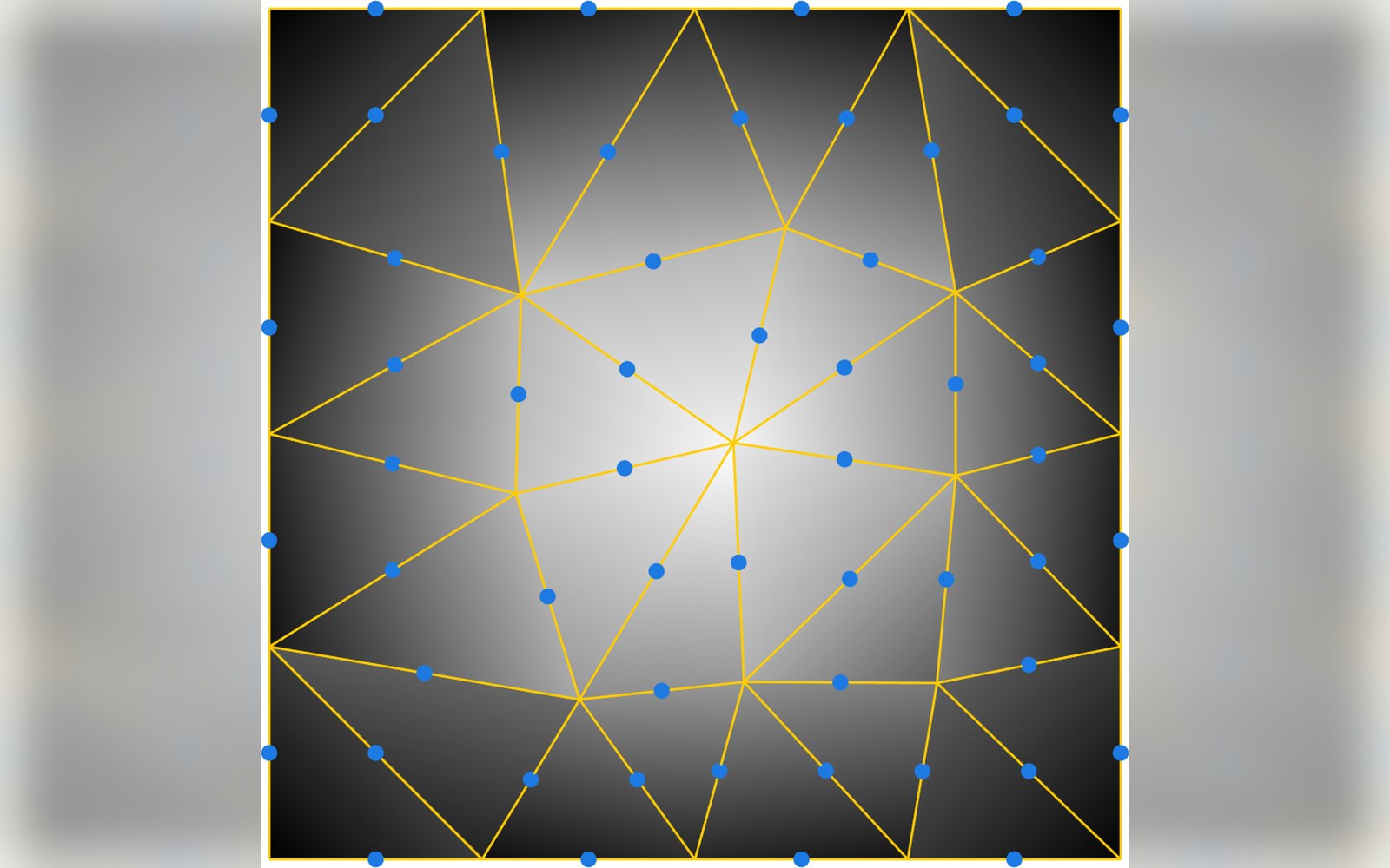
Each function is unity at its own node and zero at all others, so the nodal values are the unknowns and nothing else needs storing.
Photo: Triangulation with edge midpoints · Wikimedia Commons