Direct against iterative
Conditioning, and why it bites
The condition number of a stiffness matrix is not an abstract algebraic quantity — it is a direct measure of how much punishment a solver can take before it gives a wrong answer.

A poorly conditioned system converges slowly or not at all, and mesh quality is usually the reason.
What conditioning actually measures
Solve Ku = f, perturb f slightly, and watch how badly u changes. The condition number κ(K) is the ratio of the largest to the smallest singular value of the matrix, and it bounds the relative error amplification: a perturbation of size ε in the right-hand side can produce an error of size κε in the solution. For a well-conditioned system κ is close to one. For the systems that come out of real finite element models on real geometry, κ can reach 10⁸ or higher — meaning that eight decimal digits of input precision buy you nothing at the output.
The number is not fixed by physics alone. It depends on the element types, the boundary conditions, and, critically, the mesh. This is where conditioning bites most practitioners: a geometrically poor element degrades the system directly. The Jacobian of the isoparametric mapping enters the element stiffness integral, and when an element is highly distorted that Jacobian becomes nearly singular, pushing extreme eigenvalues into the assembled global matrix. Aspect ratio is the most familiar offender — a sliver element with edges differing by three orders of magnitude contributes stiffness coefficients that differ by the same orders, and those differences end up on the diagonal of K alongside entries from well-proportioned neighbours.
Why it matters for iterative solvers
Direct solvers factorise the matrix and live with fill-in; a badly conditioned matrix slows them through numerical cancellation but rarely fails outright. Iterative Krylov methods — conjugate gradient, GMRES — are more sensitive. Their convergence rate depends explicitly on the spectrum of the matrix: conjugate gradient on a symmetric positive definite system converges in at most n steps in exact arithmetic, but the actual iteration count tracks √κ. A jump from κ = 10⁴ to κ = 10⁸ multiplies the iteration count by roughly a hundred in the worst case and, in finite-precision arithmetic, the method can simply stall.
This is why preconditioning exists. A preconditioner M ≈ K transforms the system so that M⁻¹Ku = M⁻¹f has a condition number far smaller than the original. Incomplete LU factorisation, algebraic multigrid, and domain-decomposition preconditioners each attack the spectrum differently. Algebraic multigrid — the family descending from the work formalised through the 1980s and 1990s by Brandt, Ruge, and Stüben — is particularly effective for elliptic problems because it implicitly constructs a hierarchy that smooths both high- and low-frequency error components. But no preconditioner rescues a mesh so distorted that the underlying stiffness matrix has near-zero pivots; at that point the geometry must be fixed, not the algebra.

The condition number sets how fast a Krylov method can converge, and a few badly shaped elements are enough to move it by orders of magnitude.
What changes with material contrast
Mesh quality is not the only source of ill-conditioning. Problems with large material property contrasts — a stiff inclusion inside a compliant matrix, a thin metal liner bonded to foam — produce matrices whose eigenvalues spread across the range of the property ratio. A steel-to-rubber stiffness ratio of 10⁵ appears directly in κ. The same preconditioners apply, but they need to be informed about the heterogeneity; a preconditioner built without awareness of a stiff sub-domain will under-resolve it and leave large residuals ↗ concentrated exactly there. This interplay between geometry, material, and algebra is why conditioning is not a solver problem with a solver solution — it is a modelling problem that shows up in the solver.
This is where conditioning bites most practitioners: a geometrically poor element degrades the system directly.
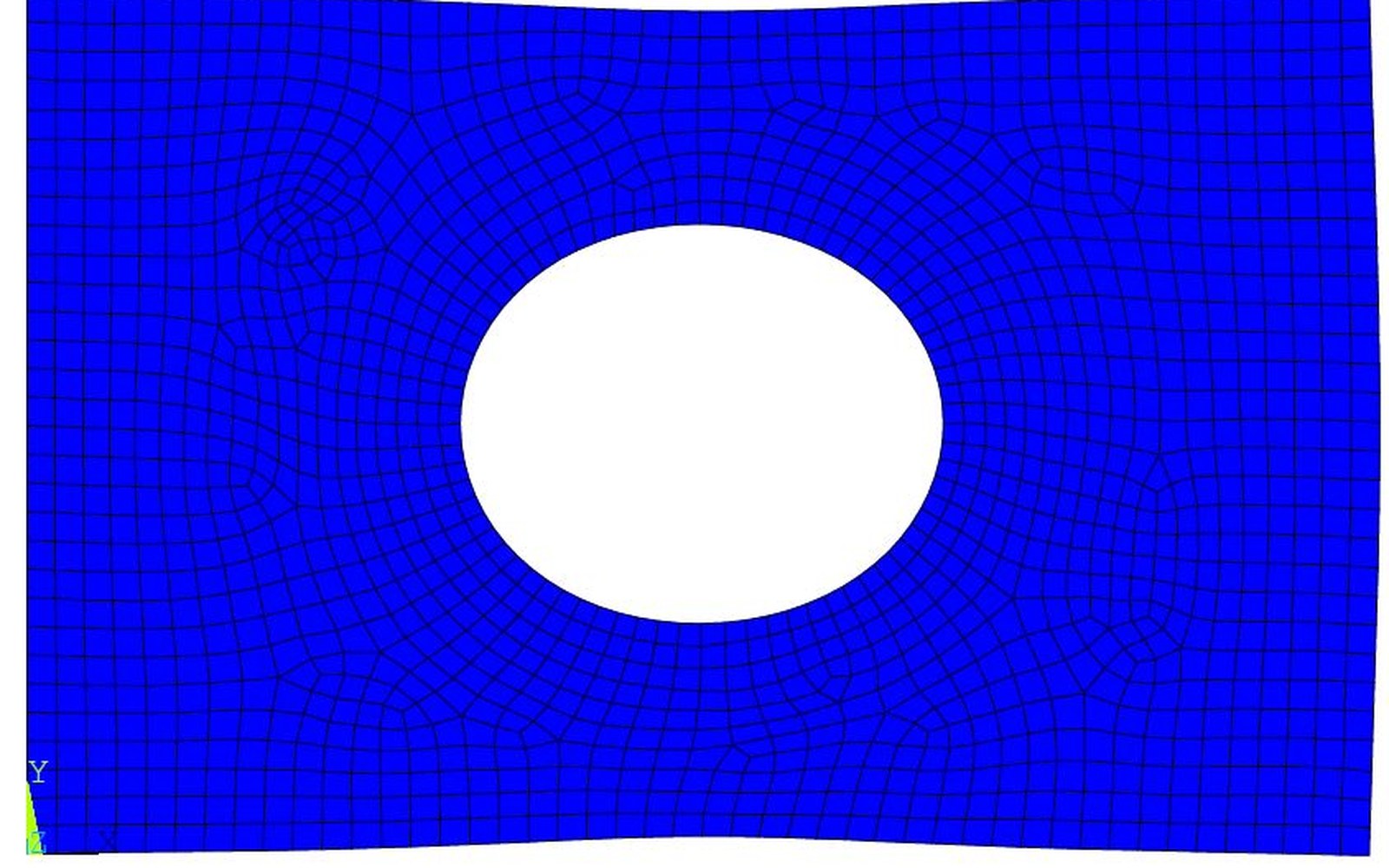
Mesh quality is the most common source of conditioning trouble, which is why the meshing argument and the solver argument are the same argument.
Photo: Meshing in Finite Element Analysis · Wikimedia Commons